Set theory and foundations of math

The following section is from the archives (lol, February 2024, which as of writing was 6 months ago. Remarkable how much I've changed.)

The goal of this original version was just to get comfortable with sets and the idea of sets, their notation, etc. — I didn't really know what I was doing when I got started, and I was (understandably, at the time) afraid of textbooks. What you're seeing for a number of paragraphs below is younger me's style, younger me's knowledge, etc.; this explains the departure in style, or something. (One thing I ran into was that I was using the wrong textbook, lol — perhaps this explains why I was afraid of the textbook)

---

We begin with Euclid, geometry -- the notion of proof.

Euclid has 5 postulates.

The fifth is the parallel postulate: An essential part of geometry as we think of it conventionally -- but if we don't accept it, we get Non-euclidean geometry, geometric systems that are formally consistent despite not representing physical space in the conventional way we might perceive it.

(something happened here and the beginning of the text got removed)

There's a parallel current going on: the need for formalization in mathematics. Before Cantor, math mostly deals with concrete, mathematical objects, and intuitions. Each part of math (e.g. geometry and arithmetic) was a distinct discipline. Take a look at, e.g. islamic mathematicians, Euclid, etc. — proofs are like paragraphs, with minimal formal notation.

Newton and Leibniz developed calculus, but didn't really formalize it — e.g. they used the notion of the infinitesimal, which worked, but wasn't formally comprehensible. So there's a desire among mathematicians around this time to formalize infinity, to avoid worries about infinite series, functions, limits, etc. having paradoxes. (This desire also probably stems from the desire to generalize and unify math into a coherent, interlinked discipline, as opposed to a bunch of different areas of study with no connection.)

In a paper, "On a Property of the Collection of All Real Algebraic Numbers," Cantor introduced the theory of sets. Sets can contain any kind of object — sets, numbers, etc. That gives them the potential to unify all the different branches of mathematics. Sets also provide an environment to formally deal with infinity — different notions of infinity, and ways to deal with it.

Set: A collection of distinct objects. E.g. $A = \{1, 2, 3\}$. The symbol $\in$ ("in") expresses membership of a set (e.g. $1 \in A$ )

Subset: Set B is a subset ($\subseteq$) of A if every element contained in B is also in A. Set B is a proper subset ($\subset$) if $B \neq A$.

• $B = \{2, 3\}$, therefore $B \subset A$
• $B = \{4, 5\}$, therefore $B \not\subset A$
• $C = \{1,2,3\}$ therefore $C \subseteq A$ but $C \not \subset A$.

Sets are not like a folder/hierarchy kind of thing. It's not that $A$ contains only $B$ if $B$ is a subset, and $B$ contains the elements; containment is not like files on a computer. Subsets are just selections of items from the set.

The empty set: written as $\varnothing$ or just $\{\}$, the empty set just doesn't have anything in it. (The set equivalent to the number zero.)

The Power set of set $A$, written as $\mathcal{P}(A)$ , is the set of all possible subsets of $A$, including $A$ itself and $\varnothing$.

For example, given that $$A = \{0, 1, 2\},$$ we can say that $$\mathcal{P}(A) = \{\varnothing, \{0\}, \{1\}, \{2\}, \{0, 1\}, \{1, 2\}, \{0, 2\}, \{0, 1, 2\}\}$$ Think of this as all possible ways to group the elements in set A: to make each subset you're allowed to take any number of items from A, however you choose. (You can't add extra elements, though.)

Cardinality: How many elements are in a set E.g. $A = \{1, 2, 3\}$, therefore $|A| = 3$

Cardinality will be an integer if the set is finite — if the set is infinite, though, it gets more complicated.

Cardinality is also related to notions of bijection, correspondence, etc. which I'll get to in a sec. Real quick, though, a cool thing to note: the cardinality of $\mathcal{P}(A)$ will always be equal to $2^{|A|}$. This is Cantor's theorem, which we'll see in a moment.

This may seem unintuitive at first (why two?) but if you think about it, it makes sense; there are $|A|$ elements, and for each subset, each element in $A$ can either be included or not included. (It's a binary choice.) Imagine selecting or not selecting items as a binary tree.

We need one more key idea to start talking about infinite cardinality: relationships between elements in sets — a special kind of correspondence called a Bijection.

Set $A$ has a bijection with Set $B$ if each element in $A$ has exactly one corresponding element in set $B$.

To illustrate, imagine we take a random element in set $A$. Now let's take a random element in $B$, and draw a line connecting the two. Keep drawing lines from one un-connected element to another un-connected element until we can't draw any more lines. If there are no elements left un-connected in either set, there's a bijection between them; if there are elements left over that don't have a pair, the sets are not bijective.

The formal way we talk about bijection defines it as a function that maps one set onto another: We define a function $f$ that maps (mapping is just the formal way to talk about drawing lines) set $A$ onto set $B$ as follows: $$f : A \rightarrow B$$ The function $f$ is bijective if $$\forall b \in B$$ — "for all elements (labeled $b$) in the set B" — $$\exists ! a \in A$$ — "there exists exactly one element in A" — such that $$f(a) = b$$ ("if you put $a$ into $f$, you get an element $b$ as an output").

How does this relate to cardinality? If two sets are bijective, they must have the same cardinality. If they have the same cardinality, they must be bijective. The same number of elements in each guarantees that you'll be able to draw an arrow between the two.

There are more kinds of -jections (injection, surjection). For $f: X → Y$:

• $f$ is surjective or onto if each $y \in Y$ has a corresponding $x \in X$ such that $f(x) = y$
• $f$ is injective or one-to-one if $f(x_1) = f(x_2) \implies x_1 = x_2$ for $x_1, x_2 \in X$ . In other words, it's one-to-one if, for any given $y \in Y$, there is only one element of the set $X$ that maps onto it.
• $f$ is bijective if it's both injective and surjective; each $y \in Y$ has exactly one $x \in X$ such that $f(x)=y$.

I'm going to use the symbol $\cong$ for bijection in this post.

To add a little bit of vocabulary, just on the side, Equinumerosity is what we call it when there's a bijection between two sets, or alternatively $|A|=|B|$ . (I think these are the same thing.)

(You might also see the term Isomorphism being thrown around; I avoid that term here even though it's technically maybe usable because the same two sets can be labeled isomorphic or not isomorphic depending on what characteristics you're looking at. Isomorphic might imply some sort of ordering relation. e.g. this video)

Let's talk now about how set theory works with infinities.

Set theory and infinity

One of the cool things that set theory lets us do is talk about different kinds of infinity. But to talk about infinity, we need a bit of vocabulary about number systems and infinity.

First, a quick review of important sets:

The natural numbers, $\mathbb{N}$, are the numbers that we count with "naturally" — they're basically the most basic idea of numbers. You can list them out in order: $\mathbb{N} = \{1, 2, 3, 4, 5 ...\}$

The integers, $\mathbb{Z}$ (just by convention I guess), are all the whole numbers. They stretch out on both sides of 0: $\mathbb{z} = \{... -3, -2, -1, 0, 1, 2, 3, ...\}$

The real numbers, $\mathbb{R}$, are all the numbers that we might normally talk about. This contains all the natural numbers, 0, fractions, infinite decimals, etc. Any normal "number" you might operate with in reality is a real number. You can't list out the real numbers in order — where do you start? 0? then what? 0.1, or 0.001, or 0.0000000001? or 1? (see more at Varsity Tutors)

Something else we'll need: ordering.

Sets don't have an order, necessarily. If you put apple, orange, and banana into a set, that concept of "order" doesn't make sense, unless you define a relation by which they can be ordered, e.g. "alphabetical order. Then the concept of order makes sense. Hence, order can be a property of some sets.

One relevant formal concept is that of a Well-ordered set. A set is well-ordered if every possible subset of it has a smallest element. For example, the natural numbers are well-ordered, because there's no way to define a subset of them that doesn't have a smallest element. (Try it!)

The real numbers $\mathbb{R}$ are not well-ordered, because we can define a subset that does not have a least element, for example, the interval of all numbers between $(0,1)$.

Well-ordered sets use the relation $<$, less than. There are other orderings of sets, though, which allow for flexibility using different operations. They get pretty complicated, but for example lexicographic ordering for letters turns $\{b,g,f,a\}$ into $\{a,b,f,g\}$ (since "less than" doesn't make sense for letters). Most of the time we'll be using $<$ though.

Ok, now we can actually get to infinity. here are lots of different kinds of infinity. One easy distinction between kinds of infinity is where we talk about countable and uncountable infinity.

We talked about this earlier with the naturals and the reals ($\mathbb{N}$ and $\mathbb{R}$) — you can count out the naturals. Start at 1, just keep going — versus with $\mathbb{R}$, we don't know where to go next; there's no sense of order.

Formally, we actually use $\mathbb{N}$ in some of our definitions for infinite cardinality. The simplest kind of infinite cardinality is countable infinity: there's no limit to the amount of elements in the set, but you can list them out in some meaningful order. A set is countably infinite if we can draw a bijection between it and the natural numbers: $$ A \cong \mathbb{N}$$ We denote the cardinality of $\mathbb{N}$ as $\aleph_0$ ("aleph null", a hebrew letter — don't ask me why, maybe they just used it cause it looks like N lol). I.e. $|\mathbb{N}| = \aleph_0$ A nicer way to say that there's a bijection between $A$ and $\mathbb{N}$ is to talk about it in terms of cardinality of N: $$|A| = \aleph_0$$

You can think about this also as "numbering" all the elements in $A$. If they have a bijective relationship, that means you could give a number to each element in $A$; e.g. you could select an element in $A$ and number it 1, then choose a different element in a and call it number 2, and continue on in this fashion infinitely.

The key idea here is that there must be a systematic way, some sort of algorithm to do this — you can't just select random elements, otherwise $\mathbb{R}$ would have cardinality $\aleph_0$, which would make the concept useless and defeat the point of distinguishing countable and uncountable infinity.

For example, we can prove that $\mathbb{Z}$ (the integers, if you remember) is countably infinite because there's an algorithm that maps every element in $\mathbb{Z}$ onto another element in $\mathbb{N}$. One way to do this is using odd and even: zero maps onto zero, then each negative number in $\mathbb{Z}$ maps onto each odd number in $\mathbb{N}$ (e.g. $-1 \rightarrow 1$, then -$2 \rightarrow 3$, then $-3 \rightarrow 5$, and $-4 \rightarrow 7$, etc.) and each positive number maps onto each even number ($1 \rightarrow 2$, then $2 \rightarrow 4$, then $4 \rightarrow 6$, etc.)

Hopefully this idea of mapping $A$ onto $\mathbb{N}$ makes sense, but if not I don't think it's essential.

Now, it seems intuitive that $|\mathbb{R}| > \aleph_0$ — there's some idea of, like, "bigger-ness" in the real numbers. There's just more of them, they don't really make sense, you can't map them onto $\mathbb{N}$. But how do we prove this?

Cantor came up with a cool method in order to prove that $|\mathbb{R}| \not = \aleph_0$, called Diagonalization. Diagonalization generalizes in all sorts of cool ways, but for now I'm going to give you just this one argument.

Let's assume for a moment that $|\mathbb{R}| = \aleph_0$ . This means that we can write out all the elements in $\mathbb{R}$ in an ordered list. For simplicity, we'll look at just a subset of $\mathbb{R}$: we'll use the numbers between 0 and 1 — if these numbers aren't countable, then since they're a subset of $\mathbb{R}$, $\mathbb{R}$ isn't countable either.

(For finite decimals we'll just add add 0s on the end to make them the same length as our infinite decimals.)

I'm going to use just some random numbers for illustration:

Index	Number	.	.	.	.	.	.
1	0.	1	0	0	0	0	...
2	0.	7	7	7	7	7	...
3	0.	7	1	8	2	8	...
4	0.	1	0	2	0	1	...
5	0.	9	9	0	0	0	...
6	0.	3	9	8	4	6	...
...	...	...	...	...	...	...	..

(Using a markdown table is hard for this visually, sorry, so feel free to watch this video version created by Trefor Bazett or just search "diagonalization argument demonstration" or something like that online. I'm sure that there are plenty of other representations out there, this is just one that works well enough and which I found within like 5 minutes of searching.)

Let's assume that we have every single possible number in this list. If we can come up with a new number that isn't in our list somehow, we prove that there would be a logical contradiction created if $\mathbb{R}$ were countable, and therefore that it cannot be countable.

Turns out, there is a way. Let's do something clever. Let's select the digits going diagonally down the list, i.e. the 1st digit of the 1st number, 2nd digit of the 2nd number, etc. going down the whole list (so that there is a digit selected from every single number in the list)

Index	Number
1	0.	[1]	0	0	0	0	...
2	0.	7	[7]	7	7	7	...
3	0.	7	1	[8]	2	8	...
4	0.	1	0	2	[0]	1	...
5	0.	9	9	0	0	[0]	...
6	0.	3	9	8	4	6	...
...	...	...	...	...	...	...

And let's add 1 to each value, turning 1 into 2, 5 into 6, and 9 into 0 (just rolling over instead of turning into 10).

Index	Number
1	0.	[2]	0	0	0	0	...
2	0.	7	[8]	7	7	7	...
3	0.	7	1	[9]	2	8	...
4	0.	1	0	2	[1]	1	...
5	0.	9	9	0	0	[1]	...
6	0.	3	9	8	4	6	...
...	...	...	...	...	...	...

There's our new number, 0.28911... and it can't be in the list already. It is guaranteed to have at least 1 place value different from every single number in the list, since we generated it by taking a digit from every number from the list and adding 1 to the digit. Its 1st digit is different from the first number on the list, 2nd digit different from the 2nd, 3rd different from the 3rd, et cetera.

Hence, we've created a contradiction. We said we had all the real numbers between 0 and 1 in our countable list, but then turned out that no matter how we list the numbers, we can always come up with a number that's not in our list. Turns out our list isn't countable after all.

Since our premise that $|\mathbb{R}| = \aleph_0$ led to a contradiction, our premise must be false; therefore $|\mathbb{R}| \not= \aleph_0$

Diagonalization will reappear in all sorts of ways down the line, in everything from Russell's paradox to Godel's Incompleteness Theorems to Alan Turing's Halting problem. Diagonalization gets really abstract, though, so I think the best way to get to that abstraction is through seeing a bunch of examples, and then coming back and figuring out what they all have in common. So for now, we'll leave diagonalization. :)

How do we compare the sizes of infinities?

We need notation and concepts to deal with different kinds of infinity. One of Cantor's most important contributions to math was his ideas about transfinite numbers, numbers that were meaningfully different in size but all bigger than the natural numbers — so infinite, but in different ways. Let's see what that means.

Let's start with Cardinal numbers. Every set has a cardinality — but when we have, say, uncountably infinite sets and countably infinite sets, we need to be able to express that. The size of those infinities is different.

We've already seen $\aleph_0$: the size of $\mathbb{N}$. $\aleph_0$ is the smallest countable cardinal; in other words, it's the smallest infinity.

$\aleph_1$ is the smallest uncountable cardinal. In other words, it's the smallest uncountable infinity. The Continuum Hypothesis posits that $|\mathbb{R}| = |\mathbb{C}|$ = $\aleph_1$ — but as of now it's unproven. We're not quite sure which $\aleph$ it is. (Understanding why this is will probably mean that you understand cardinals.)

Let's go back to our example, $\mathbb{N} \cup \{0\}$. The cardinality of $\mathbb{N}$ is $\aleph_0$. Adding one more number into that set will not change its already-infinite cardinality. We can prove this by defining a function $f$ that maps $\mathbb{N}$ onto $\mathbb{N} \cup \{0\}$; intuitively, $f$ is a bijection between the two sets. Their cardinality is the same, because we can draw a 1-1 correspondence between element $n$ in $\mathbb{N}$ and $n-1$ in $\mathbb{N} \cup \{0\}$.

But we still need to be able to talk about the individual indexes — because if we insert $0$ at the end of the set, what index would have? How do we talk about where in the set it is? For this we need ordinal numbers.

Cantor defined $\omega$, the number after all the natural numbers have been counted. You go, $1,2,3,4\ldots, \omega, \omega + 1$, etc.

If we define a set $\mathbb{N} \cup \{0\}$, $0$ would be at the $\omega$-th place in the set — after all the natural numbers have been counted. It's important now to distinguish between order and size — ordinals and cardinals. $\omega + 1$ isn't bigger than $\omega$, it just comes after $\omega$.

Ok, now let's see how far we can go now that we have $\omega$. $\omega, \omega +1, \omega +2, ..., \omega + \omega$ ($\omega + \omega$ makes sense intuitively as the union between two sets with cardinality $\aleph_0$, say, "count all the even numbers, and then count all the odd numbers."). We can rewrite $\omega + \omega$ as $2\omega$ for shorthand.

Then we can keep going, past $3\omega, 4\omega, ... \omega * \omega$. ($\omega * \omega$ = $\omega^2$; we can imagine this intuitively as a countably infinite list of countable infinities.)

Visualize $\omega^2$ as a 2d list $\omega$ by $\omega$. An infinite list of infinite lists.

Visualize $\omega^3$ as a list of those 2d lists, now extending into 3 dimensions, $\omega$ by $\omega$ by $\omega$. An infinite list of infinite lists of infinite lists.

We can't really visualize $\omega^{\omega}$, but in theory this should sorta make sense; an $\omega$ -dimensional grid of $\omega$ by $\omega$ by $\omega$ by $\omega$ by ... by $\omega$. An infinite list of infinite lists of infinite lists of infinite lists... infinitely nested.

It no longer really makes sense to visualize past this, but we can go to $\omega^{\omega^{\omega^\omega...}}$ , applying this operation infinitely. Past that we hit $\epsilon_0$.

---

Here ends the original passages of these notes from February 2024. I'm continuing on now from where I left off, ish, but mostly focusing on what is interesting.

Diagonalization

The diagonal lemma establishes self-referential sentences that you can use to prove Godel and Tarski's theorems. Huh?

• in theories that are strong enough to represent all computable functions
  • TURING MACHINES?
• Then you can use these sentences to prove godel and tarksi theorems. WTF? HUH?

Let $$\vdash_T$$ It's provable in the theory T

that for all y

the numeral corresponding to the function $f(n) = y$

bidirectionally implies the existence of a graph formula with the numeral... This isn't making sense.

. . .

We kind of have to get into first order logic here. (sources: most of this stuff is a variation on wikipedia.)

First-order logic is a nice little structure built on propositional logic. Propositional logic does simple propositions; first order logic allows you to do things like "for all" (quantification) and "x has the property y" (predicates, though I'm not really confident on that example).

For example, in propositional logic, you have to treat "that tree is green" and "the sky is green" as two wholly distinct and unrelated propositions, $p$ and $q$. Propositional logic can only deal with logical objects, like those propositions — they have to be true or false. On the other hand, in first-order logic you can use logical properties to work with non-logical objects, e.g. call that tree $x$ and call the sky $y$ and express the aforementioned propositions as $\text{isGreen}(x)$ and $\text{isGreen}(y)$. We're applying the predicate $\text{isGreen}$ to particular objects, which themselves don't have to be logical, e.g. trees. We call these things "formulas": basically statements of logical relations, or something like that.

Obviously you need to be able to formally define the criteria for evaluating the predicate's truth or falsehood, but in principle this is more powerful and lets us set up cooler systems or something.

You can also establish other kinds of formulas. You can establish relationships between predicates with logical connectives (e.g. and, or, if/then [aka "implies"]) e.g. "if $x$ is green, then $x$ is alive" $$G(x) \implies A(x).$$ You can quantify variables, e.g. "for all $x$, if $x$ is green, then $x$ is alive." $$(\forall x )[G(x) \implies A(x)]$$ An "interpretation" or "model" of a formula specifies what all of it means — rules for interpretation. (There's no correspondence between description modes or programming languages here, is there? Wait, yes there is — programming language compilers tell the computer how to relate the formal symbols to the "outside world," the memory and everything. Interpretations or models connect the symbols to the rules for computation. This is very much the same thing. The analogy for description modes is a little bit weirder but it's there? Maybe? Description modes are rules for decompression — a little more abstract but the idea of "interpretation" or "rules for relation" holds.)

The rules for interpretation tell you what the predicates mean, and what the "entities" are that can make them true or false (Wikipedia says "instantiate the variables"), forming the domain of discourse: the set containing all the things you're talking about. (Huh? Naive set theory moment?)

For example, in an interpretation with the domain of discourse consisting of all human beings and the predicate "is a philosopher" understood as "was the author of the Republic", the sentence "There exists $x$ such that $x$ is a philosopher" is seen as being true.

There's lots of random shit going on in the wikipedia page for syntax. ~~I wonder whether this work is actually substantive progress, all these definitions, or if it's just sort of obscuring other problems.~~

Returning to the sentence above: $$\vdash_T (\forall y)[(^\circ f(n) = y) \Leftrightarrow \mathcal{G}_f(^\circ n,y)]$$A couple things that stuck me at first. The notation $\vdash_T$ here, just to have full clarity, is saying "the following statement has a formal proof in the (first-order, in this case) theory $T$." $\mathcal{G}$ is referred to as a "graph" formula or something. Claude explains this as $\mathcal{G}$ being a way of representing a function in terms of input-output pairs ($x$ and $y$) where $y = f(x)$. This is convenient because it allows us to treat $f$ as a black box, knowing its inputs and outputs but not knowing what goes on inside it, if anything. Additionally, since we're working within this specific theory $T$, we can't just access numbers (the real things??)(???¹), instead we just work with numerals that correspond to the numbers. (The numbers are in the domain of discourse, here — since they're from the meta-theory, which is what mathematicians call the real world 😎). That's what the $^\circ$ indicates.

The way we typically define numbers in basic formal systems is using a successor operation $S$. Putting that together with the numerals stuff, and assuming that Claude is reliable on this point(?), we're looking at something like, "what we call 0, the number, is represented by the numeral $^\circ 0$", "1 is $S(^\circ 0)$", "2 is $S(S(^\circ 0))$", et cetera. This notation is important so we don't get confused while doing meta-mathematics and such.

Bringing it back to the sentence:

$$\vdash_T (\forall y)[(^\circ f(n) = y) \Leftrightarrow \mathcal{G}_f(^\circ n,y)]$$ "it is provable in theory $T$ that, for all $y$, the statement the $^\circ f(n) = y$ is true if and only if i.e. the formula $\mathcal{G}_f (^\circ n, y)$ is provable (i.e. the graph function we defined for $f$ maps $^\circ n$ onto $y$)."

This sentence is asking, "Does $\mathcal{G}_f$ accurately capture the behavior of $f$ in the way that we would expect a graph function to?" It's important because we're taking a function $f$ from outside this theory $T$ — $f$ operates on actual numbers, whereas $T$ can only operate on the representations — and bringing it in using a graph formula.

I don't really understand this very well. I think I'm confused about the whole idea of what's going on here — why does it matter that we can capture the behavior of some outside function? I'll hold that question and see if it gets answered as I continue reading. For now, I'll leave it as "We need this way of bringing outside functions into our first-order theory for now."

We also need a way of assigning Gödel numberings to our formulas as labels.

Gödel numbering

A simple way to do this would be quite reminiscent of when we were talking about binary encodings. We could use ASCII, even — represent our functions in ASCII with (to take Wikipedia's example) x=y => y=x represented as 120 061 121 032 061 062 032 121 061 120. You could concatenate them and there's a unique integer.

Gödel didn't do it like this, cause it limits your vocabulary to however large your coding range (for ASCII, 127 distinct characters). There's a nicer way to do this that has an infinite vocabulary size — it can incorporate as many distinct symbols as you'd like! The cheat code: there are infinite primes. You can assign a prime number to each symbol you want to represent, and then create a coding based on that.

Why not just append these prime numbers and call that the Gödel number? Well, you could, but it wouldn't be guaranteed to be unique. For example, if you had a symbol corresponding to 13 and a different one corresponding to 1, as well as one corresponding to 131 (which you likely would, since 131 is a relatively small prime) you wouldn't be able to tell the difference between 131 ($\text{append}(13, 1)$) and 131 (the symbol corresponding to the prime number 131) when decoding. You could add spaces to your encoding, but that would just be un-elegant and lame and wouldn't actually be a unique number, it would be some weird thing with spaces in it that isn't a number. (You could replaces the spaces with 9s or something maybe, but even that might not be guaranteed to be unique. Also it would be lame and un-elegant.)

What Gödel did instead was assign each position in the sequence a corresponding prime number (greater than two), and then raised them to the power of the symbol in that position — so it would look like $$2^{x_1} \times 3^{x_2} \times 5^{x_3} ...$$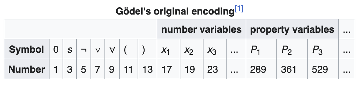This works because a number's prime factorization will always be unique, and the power of each prime will always be recoverable. There are other more sophisticated ways to do this but Gödel's original technique seems to be good enough to cover the idea.

Now, returning to the sentence we discussed earlier with this in mind. We can assign every formula a natural number this way; we can call it a function $\#$ that maps formulas onto numbers or something. The notation we can use for this is assigning formula $\mathcal{A}$ a natural number $\#(\mathcal{A})$. Within $T$, these assignments will be $^\circ \#(\mathcal{A})$ (since they're the numerals corresponding to that number).

Prove the diagonal lemma

This is actually something I'm not prepared to do yet! I spent about two and a half hours trying to grok the proof of the diagonal lemma today, and while I think I made some intuitional advances, there are too many underlying conceptual gaps that I'm missing to be able to do this at this point. I don't currently have enough experience with first-order logic to feel comfortable speaking its language; there are too many things that I don't currently understand for this to be successful. Some gaps in my knowledge I'm hitting:

• Difference between predicates and functions — I think I have some sense of this but it's weak and doesn't have enough concrete practice. I think just general comfort with first-order logic and formal evaluation is an issue; I have some comfort with propositional logic but it hasn't translated well. (This is the type of thing that I think college courses and textbooks do well.)
• How Gödel coding actually encodes predicates, also free variables in general: The thing that is especially tripping me up is the notion of a free variable, and how it looks in the Gödel coding. (I attempted to explain it in footnote ² if you would like to see the current status.) I need to write out or see more examples of how Gödel coding works.
• Comfort with the notion of numerals vs. the numbers they represent
• Standardized notation: I don't have a good grasp of what standard notation looks like.
• Lack of easy consistency between resources: my typical method of learning is cross-referencing lots of different sources (usually online resources, or a textbook that I went through the effort to obtain) that match each other notationally.² tried doing this with Wikipedia, Math Stack Exchange, and LLMs, but they have different approaches that don't easily map onto one another. Also, Claude kept hallucinating which was a big problem.

All in all I think I developed a lot of useful knowledge in attempting this — it was fun and ambitious and I got a taste for the thing that I really want to hit at the end of this. I think if I tried again I might be able to get it, but instead of trying online resources I'd cross-reference a textbook with these notes; I'd skim the buildup in the textbook and try and anchor myself in where I can look when I get stuck; and I'd set up a two-agent critique setup where GPT-4o and Claude critique one another to (hopefully) limit hallucinations.

I'm archiving my failed attempts here as a public reminder that learning is kinda hard, and also as a reminder to myself that feeling stupid is okay sometimes and is a natural step in figuring new things out from scratch. I have given them to you in plaintext cause I don't want you to actually read them, lol, and also because I don't want someone to mistake them for "things I actually think are mostly correct" if they're skimming the page and don't see this header/disclaimer section you're reading right now. If you really want to read them, you can copy-paste them to a markdown editor and fix some of the web-specific LaTeX rendering if you want to view it properly. (I had to backslash escape some of the LaTeX, specifically parst that contained \# (so I'd double backslash it) or _, so that it would render correctly with MathJaX.)

Attempt 1:

*(I'm continuing to just work from [Wikipedia](https://en.wikipedia.org/wiki/Diagonal_lemma) here,  adding my own explanations as I understand things.)* 
The lemma looks like this: $$\vdash_T \mathcal{C} \Leftrightarrow \mathcal{F}(^\circ \\#\mathcal{c}).$$ $\mathcal{C}$ is a self-referential sentence: it says that there is some property $\mathcal{F}$ that applies to the numeral corresponding to the natural number corresponding to its own Gödel coding. The lemma doesn't specify what $\mathcal{F}$ is, it's just an arbitrary formula; its proof doesn't depend on the meaning. 
To prove the diagonal lemma, you first introduce a function $f: \mathbb{N} → \mathbb{N}$ that takes in a natural number, sticks it into the formula $\mathcal{A}$, and then gives it a Gödel coding: $$f(x) = \\#(\mathcal{A}(x))$$For some natural number $x$ and any formula $\mathcal{A}(x)$. ("substitute $x$ into $\mathcal{A}$ and then give it a Gödel coding.") 
Then, since $\mathcal{A}(x)$ now has a Gödel coding, we can plug that natural number (Gödel coding) into $f$. $$f(\\#\_{\mathcal{A}(x)}) = \\#[\mathcal{A}(^\circ \\#\_{\mathcal{A}(x)})]$$ We assume that the Gödel coding function $f$ is computable (which it almost always is? I think?), and using our statement from above, we can create a graph function for it. 
Since it's a theorem that for a computable function $h$, $(\forall y)[(^\circ h(n) = y) \Leftrightarrow \mathcal{G}\_h(^\circ n,y)]$ (this is the statement we used above, just swapping some characters to avoid confusion) we can create a graph function $\mathcal{G}\_f$ for our Gödel coding function $f$: $$\vdash\_T (\forall y)[(^\circ f(\\#\_{\mathcal{A}(x)}) = y) \Leftrightarrow \mathcal{G}\_f(^\circ \\#\_{\mathcal{A}(x)},y)].$$ 
Now, we can define $\mathcal{B}(z)$ as that the graph function... I'm running out of steam. I don't feel like I can understand this.

Attempt 2:

**Let's try a different version of the same proof.** Here I'm taking from [Stack Overflow](https://math.stackexchange.com/questions/127852/unpacking-the-diagonal-lemma?rq=1), using different notation that Claude used natively:
$$T \vdash \psi \Leftrightarrow \phi(\ulcorner\psi\urcorner)$$
$\ulcorner\psi\urcorner$ is the Gödel coding of the formula $\psi$ (psi). In our theory $T$, the formula $\phi(\ulcorner\psi\urcorner)$ ($\phi$ = "phi") is proven to be true if and only if the formula $\psi$ is true; the same opposite relation holds, where $\psi$ is only true if $\phi(\ulcorner \psi \urcorner)$ is true. This is therefore in a sense a "truth-checker function." We want to prove the existence of this function.
First, we define a function $\text{diag}(x)$:$$\text{diag}(x):=\ulcorner\xi_x(^\circ x)\urcorner.$$$\text{diag}$ takes in a natural number $x$, which corresponds to some formula $\xi_x$. It plugs the numeral version of the Gödel encoding for $\xi_x$ into the formula for $\xi_x$. We call this "diagonalizing $x$."
Okay, now we define another formula $\delta$ (delta) such that $$\delta(x) := \phi(\text{diag}(x)).$$$\delta$ is just taking a diagonalization and wrapping it in some arbitrary formula $\phi$ which we care about. $\phi$ is a predicate, a property or something like it — e.g. $\phi(x)$ could be "$x$ is even" or "$x$ is prime". What we're doing with $\delta$ is creating a self-referential version of $\phi$ that we can use; that's why compose $\phi$ with the diagonalization of some unknown input $x$. You can think of $\phi(\text{diag}(x))$ as saying, "this diagonalized formula has some property that we care about."
Then we're going to use $\delta$ to diagonalize itself. We will call this result $\psi$: $$\psi = \delta(\ulcorner\delta\urcorner))$$Using simple algebra, we replace things with themselves to get the result $\psi = \delta(\ulcorner \delta\urcorner)\\ =\phi(\text{diag}(\ulcorner \delta\urcorner))$. Then using the definition of $\text{diag}$, $\delta$ is our function $\xi_x$ and $^\circ \ulcorner \delta \urcorner$ is our $x$. So $\text{diag}(\ulcorner \delta\urcorner)= \delta(\ulcorner \delta\urcorner)$; we can continue what we just started.
$$\begin{align} \psi & = \delta(\ulcorner \delta\urcorner)\\ &=\phi(\text{diag}(\ulcorner \delta\urcorner)) \\ &=\phi(\delta(\ulcorner \delta\urcorner)) \\ &=\phi(\psi) \end{align}$$
and there we have the sentence we wanted, $\psi = \phi(\psi)$. 
Informally, we make $\phi(x)$ something like "$x$ is not the Gödel number of a provable formula"; this encodes something like "$\psi$ is provable if and only if $\psi$ is not provable." Hooray! You've encoded a contradiction!
Questions
- Why is this called a fixed-point?
- primitive recursive functions — loop a finite time. complexity class.
- peano arithmetic and robinson arithmetic. 
- Kleene's recursion theorem in computability theorem