Information theory and statistics
If you're curious about the sources for this post, they are
- Wikipedia (asking questions to LLMs about it)
- Shannon's original information theory paper
- An Introduction to Kolmogorov Complexity and Its Applications by Ming and Vitányi
What actually is information lol
It's been described to me as, "information resolves uncertainty." I think the best way to get a sense for it is talking about surprisal with regards to a specific thing.
You come to a fork in the road and you have no ideas about which way might be the correct way to go. We can represent them as paths $A$ and $B$. A natural way to represent this is with binary labels, hence it would be instead path $0$ for $A$ and path $1$ for $B$. Intuitively, if someone perfectly trustworthy tells you which way to go, they would be be giving you 1 bit (binary digit) of information: they're giving you a 0 or 1 to distinguish the options in the binary choice.
What if you do have some information preceding this, though? What if you have 70% confidence that path $A$ is correct, since someone earlier on the road who seemed somewhat trustworthy told you it was? They wouldn't be giving you still 1 bit of information, because you'd be updating less — you're less surprised. You already thought this was the case, they're just upgrading your confidence. No longer can we work with simple integers of bits; we realize from this that the amount of information you get is directly related to how much knowledge you already have — or don't have.
The intuition here is that the amount of information you're getting is related to how surprised you are to receive it.
In a formal sense, surprisal quantifies how wrong your predictions were. (At least, this is one way to think about it — a starter intuition, if you will.) When an event you didn't expect occurs — i.e. it surprises you — that surprise tells you that your model of the world was wrong or incomplete, insofar as you didn't predict the event with 99.99% confidence. Hence, you most likely have to update your internal model of the world such that it would predict that outcome with higher confidence. Surprise tells you that you're receiving information about the world, about how your model was wrong.
If you have a perfect internal world model — i.e. you're literally omniscient and you can simulate every single possible causal relation in the universe at once — your model will never update, and you'll never be surprised; you know all the information! Conversely, if your model of the world is consistently horrible, you'll be constantly updating your model after your predictions are falsified, constantly surprised at the world. You know very little of the information.
I'll talk about how to measure error and surprise soon, but for now I want to finish formalizing information — I'll derive intuitively the way you actually calculate the information you receive from an event's occurrence.
Two incorrect intuitions
I'll start with two ways that you might naturally think about information as a mathematical object, and why those ways lead you to computational problems.
From the 70%/30% situation above, you might think that the person on the path would be giving you 0.3 bits of information, thus making up for the difference in the outcomes. (This would be incorrectly applying intuitions that "probabilities should sum to 1.") If you think about this more deeply, though, the math doesn't work out; distinguishing between two perfectly uncertain options — events that have priors of 0.5 each — would only give you 0.5 bits of information, as opposed to the 1 bit we would expect. Shouldn't someone revealing to you a bit — a zero or a one, a binary choice — give you one bit of information, if you have literally no idea what that bit might be?
Here's another way that "adding to 1" doesn't work out nicely: if you have two fair coins and you flip them both separately, each coin flip would theoretically give you 0.5 bits of information. However, if you looked at it from the perspective of their joint probability distribution — for example, $P(\text{2 heads}) = 0.5 * 0.5 = 0.25$ — we would get 0.75 bits of information instead. This just straightforwardly doesn't work out. Two independent events should not give different amounts information just based on whether you look at their probabilities together or separately — but we just saw that happen! We have to keep looking.
Okay, so information for an event $x$ can't just be $1-P(x)$. What else could it be?
If we think about it, the information we get is quantifying how wrong we are. If event $x$ happens and we predicted it with very high confidence, the amount of information should be really low — we expected it, and aren't very surprised. But conversely, if we predicted $x$ with really low confidence, the amount of information should be very large — and it should scale with orders of magnitude. If our $P(x) = 10\%$ and $x$ occurs, this should be very very different from if our $P(x) = 0.1\%$ — orders of magnitude different. So maybe we could say information is proportional to $1/P(x)$?
That's almost right, but we're still missing something.
To see what's wrong let's imagine two fair dice. The probability of rolling a one on die $A$ is $1/6$; for $B$ it's also $1/6$. If we use $1/P(x)$, and look at the dice independently, seeing snake eyes — two ones — (or any other outcome for that matter) would give us $6 + 6 = 12$ bits. But if we once again consider the joint probability distribution, and ask what the probability of rolling snake eyes is, that probability is $1/6 \cdot 1/6 = 1/32$ — so if we once again rolled snake eyes, we'd get 32 bits of information instead of 12!
Information, the right way
What's going on here? We once again just combined two independent events together into one observation without changing their independence, without changing the probability — and the amount information changed. The problem is that we want information to change additively, not multiplicatively; when you "get more information" from an event your knowledge doesn't double, but increases linearly — at the same times as probability, the quantity we want to base our observations on, scales multiplicatively.
To go back to the dice scenario: when we look at the joint distribution of the two dice, or three dice, or $n$ dice, the probability of one specific combination of those dice will be $1/6^n$. But we want the information to increase linearly as the probability decreases multiplicatively. If we wanted to linearize our probability graph, what would we do?
Take the $\log$ of it!
Since we're working in binary already (with bits of information), we can use the $\log_2$ scale — our probability will be $P(x)$ and our information will be $\log_2(1/P(x))$. Ta-da! Here's our information equation: $$I[x] = \log_2(\frac{1}{P(x)}) = -\log_2(P(x))$$ (Sometimes it's nicer to use a negative sign instead of an inverse, but they're equivalent.)
To sum it up, we use $1/P(x)$ because we want information to be inversely proportional to probability — the occurrence of a (in our minds) low-probability event should give us lots of information, and the reverse for high-probability events. Then we add the $\log$ so that information will add when we look at multiple events together, instead of multiplying — it'll accumulate nicely over time instead of exponentiating rapidly.
This equation gives us nice properties:
- We get 1 bit of information from perfect uncertainty between 2 outcomes: $\log_2(1/2) = 1$
- When we are looking at the coins, the information is the same whether or not we look at the joint probability distribution. $-\log_2(0.25) = 2 (-\log(0.5))= 2$.
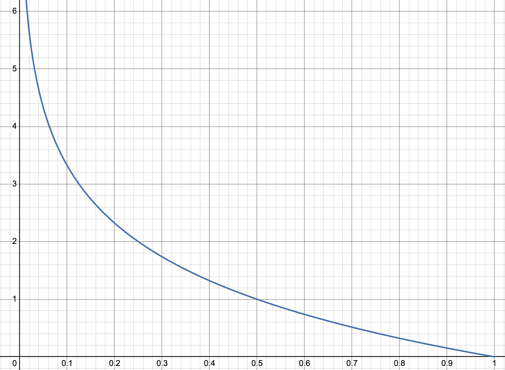 Fig 1: The graph of $y = \log_2(x)$, where $y$ is the "information content" or the surprisal produced by the occurrence of an event whose probability in your mind is $x$.
So there's the idea about why the information content of an event uses a log scale. To sum it up, $\text{Information} = -\log_2P(x)$ where $x$ is an outcome and $P(x)$ is the probability of that outcome. (Sorry to mix notations with $x$ being probability and $x$ being an outcome — hopefully that's not too annoying.)
Entropy
We might want to look at information on the level of a probability distribution. We've talked about the information content of specific events, but how do we talk about our beliefs about an event — our internal distributions?
One thing we can talk about is entropy. Entropy in information theory describes something like, "How predictable is this distribution? How surprised will I be on average by an outcome?" In general, entropy measures the predictability of a distribution. (This is not a notion limited to information theory. For example, in statistical mechanics, the entropy of a particular macrostate/thermodynamic state is the number of possible microstates that could produce that macrostate — in other words, the unpredictability of the precise arrangements of atoms for a given macrostate; the unpredictability of the particular positions of atoms, summed over the distribution of all of them.)
Intuitively, to talk about how much we expect to be surprised given a distribution of the probabilities of possible outcomes of an event, we can do a simple expected value calculation: take the sum of the information content of each possible outcome, weighted by the probability of the outcome.
Hence, we can describe "expected surprise", AKA Shannon entropy ($H$1, for a probability distribution $X$ using the following formula: $$ H(X) =\sum_{\text{all outcomes in x}} \text{P(outcome)} \cdot \text{Info if outcome occurs}$$
Written in variables: $$H(X) =\sum_{x \in X} P(x) \space \log_2 \frac{1}{P(x)}$$ or $$ H(X) =-\sum_{x \in X} P(x) \space \log_2P(x) $$ where $X$ is a distribution of individual events $x$ and $P(x)$ is the probability you assign to the event. Hence, this sum represents going across each possible event in the distribution and computing the value $P(x) * \log_2(1/P(x)$ — corresponding to the info given by an outcome, weighted by how likely it is — then summing that up for each distribution.
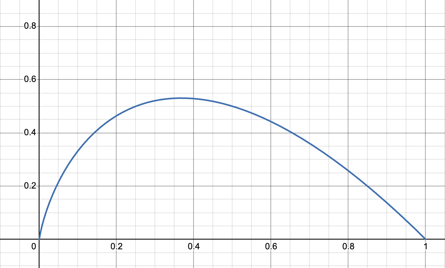 Fig 2: The graph of $-x * \log_2(x)$, which you can call the "expected surprisal" — the probability of the outcome occurring times the surprise that you would receive if it did occur. Notice how the graph is skewed right, but low-probability events, even though they have high surprisal, will have low expected surprisal because they're so unlikely.
Higher entropy to me intuitively means less predictability. For example, for the distribution $$X: \{x_1 = 0.9, x_2 = 0.05, x_3 = 0.05\}$$ the entropy is $$-[(0.9 * \log_2(0.9)) + 2 * (0.05 * \log_2(0.05)] \approx 0.473$$ — whereas for the less-predictable distribution $$X: \{x_1 = 0.33, x_2 = 0.33, x_3 = 0.34\}$$ the entropy is $$-(2 * (0.33 * \log_2(0.33)) + (0.34 * \log_2(0.34)) \approx 1.585.$$
Comparing distributions with K-L Divergence
Okay, we know how to measure the "disorder" or "unpredictability" of a distribution using its entropy. If we wanted, we could compare two distributions just using their entropy — but that wouldn't tell us how similar they were to one another. They could be entirely different, with entirely different events which had entirely different probabilities, and still have the same entropy. Our comparison would only give us a measure of how relatively disordered or unpredictable one distribution is to another.
We want a way to look at two distributions and see how different they are. For example, maybe you have reliable information about the true probability distribution for some set of events, and you want to measure how different your internal predictions were from that true distribution — say, to compare your accuracy to that of your friend's models. (I mean, you usually can't access your internal probabilities for things, so let's pretend you both actually made statistical models of the thing.)
One way to do this is Kullback–Leibler divergence, but people seem to have a hard time pronouncing this (?) so instead they just call it "KL Divergence." This comes up all the time in other fields, for example machine learning — it turns out that it's really useful to be able to compare two distributions!
The intuition for how you calculate KL divergence builds on the concept of surprise and information we built up earlier.
Let's say you want to play a coin toss game — if it's heads you win, if it's tails you lose. Your friend Anansi conveniently has a coin on hand, and offers it to you for the game. Unbeknownst to you, Anansi's coin is unfairly weighted — it's tails 70% of the time and heads only 30% of the time.
Hence, you have the following distributions:
$P$ is the true probability distribution of outcomes given by the weighting of Anansi's coin.
| Outcome | Heads | Tails |
|---|---|---|
| Probability | 0.3 | 0.7 |
$Q$ is your model of the distribution of outcomes for that coin toss. (You assume it's a fair coin by default.)
| Outcome | Heads | Tails |
|---|---|---|
| Probability | 0.5 | 0.5 |
How do we measure the difference between these two simple distributions?
One way to do this would be to measure the expected additional surprise that we'd receive from playing this game thinking that the outcomes were governed by distribution $Q$ when actually they were governed by $P$. To put it another way, we'd be measuring the additional surprise we get if we think $Q$ instead of $P$ is true.
If you're using model $Q$ when the true probability distribution is $P$, the expected additional surprise for that single event will intuitively be
- the true frequency of the event ($P(x)$)
- times the additional amount you're surprised when it happens using $Q$, relative to the amount you'd be surprised if you used $P$ instead.
Formally, you write this as $$P(x)\cdot(\ln(\frac{1}{Q(x)})-\ln(\frac{1}{P(x)}))$$ and if you want to look at this across the whole distribution (each event $x$ in the set of events $X$), you just use the summation
$$\sum_{x \in X}P(x)\cdot(\ln(\frac{1}{Q(x)})-\ln(\frac{1}{P(x)}))$$ giving you the formula for KL Divergence!
(Also, if you're confused by the use of $\ln$ instead of $\log_2$, see footnote 2. TL;DR the different logarithms don't matter much, you just kinda use whatever's convenient, so I'm switching to $\ln$ here because it's conventional for calculating KL divergence and is hence convenient.)
You might notice that this looks a lot like the entropy formula, which if you recall (now with $\ln$ instead of $log_2$) is $$H(X) =\sum_{x \in X} P(x) \space \ln \frac{1}{P(x)}$$. This similarity should make sense! Remember that entropy measures expected surprise; KL divergence measures expected additional surprise. In fact, another name for KL divergence or expected additional surprise is relative entropy! The only difference is that you're now measuring the divergence of one distribution from another, instead of just the expectations you have about a single distribution in isolation.
Great. Now we can use this to calculate the divergence of our predictions from the true probabilities of heads/tails from Anansi's coin — but first, let's adjust some things in this formula real quick, so that this definition looks like the more standard one on Wikipedia. First, we need to give it a formal function name. Standard is $D_{KL}(P \space ||\space Q)$ ("the KL divergence of P from Q"): $$D_{KL}(P \space ||\space Q) = \sum_{x \in X}P(x)\cdot(\ln(\frac{1}{Q(x)})-\ln(\frac{1}{P(x)}))$$
Then we do a bit of logarithm algebra, turning the log subtraction into division inside one logarithm:
$$D_{KL}(P \space ||\space Q) = \sum_{x \in X}P(x)\cdot\ln(\frac{\frac{1}{Q(x)}}{\frac{1}{P(x)}})$$ And then we just simplify the fraction using the reciprocals to get our final equation: $$D_{KL}(P \space ||\space Q) = \sum_{x \in X}P(x)\cdot\ln(\frac{P(x)}{Q(x)})$$ To reaffirm this intuitive derivation, let's get back to playing games with Anansi. Our expected additional surprisal for a single game would be $$\textbf{(1)} \: \: P(\text{Heads})\cdot [\ln\frac{1}{Q(\text{Heads})}-\ln\frac{1}{P(\text{Heads})}]$$$$+ \space \space \space P(\text{Tails})\cdot[\ln\frac{1}{Q(\text{Tails})}-\ln\frac{1}{P(\text{Tails})}]$$
Which we can simplify as follows:
$$\textbf{(2)} \: \: P(\text{Heads}) \cdot \ln(\frac{1/Q(\text{Heads})}{1/P(\text{Heads})}) + P(\text{Tails}) \cdot \ln(\frac{1/Q(\text{Tails})}{1/P(\text{Tails})}) $$ $$\textbf{(3)} \: \:P(\text{Heads}) \cdot \ln\frac{Q(\text{Heads})}{P(\text{Heads})} + P(\text{Tails}) \cdot \ln\frac{Q(\text{Tails})}{P(\text{Tails})} $$
Now, we can write it all in decimal form, substituting according to our two-way table
| Heads | Tails | |
|---|---|---|
| P(x) | 0.3 | 0.7 |
| Q(x) | 0.5 | 0.5 |
$$0.3 \cdot \ln(0.5/0.3)+0.7 \cdot\ln(0.5/0.7) \approx 0.08228 $$ To confirm this, we can write a little python script (credit to Zach Bobbitt on Statology):
from scipy.special import rel_entr

    P = [0.3, 0.7]
    Q = [0.5, 0.5]

    print(sum(rel_entr(P, Q)))
Which nicely yields 0.08228287850505178. :D
There's how you describe and calculate K-L divergence!
Bounds on algorithmic compression
Until now, we've mostly talked about information as it relates to surprise, or error, with events out in "the world" — you get information from "the world" when your predictions about it don't match up to reality. However, "the world" doesn't have to be, say, reality as a whole (in the style of a bayesian agent that does predictive processing/active inference, which I'll talk about in another post or something): we can zoom into specific kinds of events that are modeled by probability, and treat those as if they are our entire "world" — we just need to slightly adjust the way we apply our intuitions.
In particular, here I'm thinking about applying information theory to data transfer and compression. It's useful and interesting — though it is somewhat limited in its results, for reasons related to the assumptions of Shannon's coding theorem (in particular, that the sequence we're talking about was generated probabilistically, with each character coming from the same random variable defined by the same distribution) which I'll talk about more below. But I think this is a great starting point for lots of other interesting ideas I'd like to get to, like Kolmogorov complexity, and, surprisingly, diagonalization arguments like Gödel's incompleteness theorems.
(Note: this post was originally combined with the K-complexity and algorithmic information theory post. I split them apart because the k-complexity post naturally turned into theoretical computer science and I wanted to keep this one statistical. See the k-complexity post if the above paragraph intrigued you.
Shannon's source coding theorem: probabilistic/unstructured information
Let's say we have a probabilistic event, and we want to store a history of its occurrences. We can return to our scenario with Anansi for this.
Anansi finally told you that the coin wasn't fair, so you decided to play a game with a four-sided die that he had in his pocket instead. (A pyramidal die, basically — look it up if you've never seen a d4 before.) You'll roll the die a bunch of times and then tally up your score after 20 rolls — so you need to save the results of your rolls in a string. For convenience, the die has numbers 0 to 3 on it instead of 1 to 4.
You could store it as follows:
3 2 1 2 3 2 2 1 3 1 2 2 2 2 2 2 3 3 0 2
In a computer that would be stored in bits (spaces added for readability; in reality there are no spaces between numbers):
11 10 01 10 11 10 10 01 11 01 10 10 10 10 10 10 11 11 00 10
But let's say, for the sake of illustration, our storage space is super limited. Is there way to compress this string — any shorter representation of it that could still save it exactly?
The answer is, basically, "not really." Shannon's source coding theorem formalizes this. Source coding is what we call it when we encode the output of an information source into symbols from an alphabet, usually bits, such that it's invertible, i.e. you can undo the encoding to get the original output of the information source. For our current purposes, this information source needs to be discrete, like dice rolls or words in spoken English, not a continuous function. (You can extend these ideas to continuous functions, but that's a separate domain called rate-distortion theory, which I currently know nothing about.)
Shannon's source coding theorem states that (a) the upper bound on efficiency of compression for a discrete information source generated by a random variable is the entropy of that random variable, and (b) you can create encodings that get arbitrarily close to that bound.
Let's unpack that a bit. (A) is placing a bound on how well you can compress a sequence like the one we have above. The actual mathematical formulation says that the average number of bits per symbol can't be less than the entropy of the variable.
Let's walk through an example using the 4-sided die and our formulas from above. The entropy of our 4-sided die — assuming it's fair — is the sum over each possible outcome's probability times the information it would give us. (Note that I'm going back to $\log_2$ because we're using bit representations of the code and it's nice if we use that.)
$$ \textbf{(1)} \space \space H(\text{4-sided die}) = \sum_{x \space \in \space \text{outcomes}} P(x) \cdot \log_2 \frac{1}{P(x)}$$ $$ \textbf{(2)} \space \space H(\text{4-sided die}) = 4 (0.25 \log_2(1/0.25) $$ $$ \textbf{(3)} \space \space H(\text{4-sided die}) = \log_2(4)= 2 \: \text{bits}$$ So our entropy is 2 bits. As you saw above, we were storing our scores in two-bit numbers (spaces added for readability):
11 10 01 10 11 10 10 01 11 01 10 10 10 10 10 10 11 11 00 10
Which is great! That means we have an ideal encoding — the code rate (this is the technical term for "number of bits in the encoding, per symbol in the original source.") is 2 bits, which is equal to the entropy.
So what (a) in Shannon's source coding theorem is saying is that no matter how good our encoding is, we'll never be able to find an encoding that has a lower code rate than the entropy of the source — that is, without losing information. (If we're willing to compress lossily, we might be able to get below that bound.)
What (b) is saying is that, no matter the discrete source, we can always find an encoding that gets the code rate arbitrarily close to the source's entropy. For the situation with a fair 4-sided die, we by default have a coding that's ideal; that's usually not the case.
Back to you and Anansi. You clearly should have expected that Anansi would have an unfair die, if he already had an unfair coin on hand. After playing with him for a while, you begin to really suspect that the die isn't fair. You press him on it, and he finally reveals the true distribution of values:
| Value (x) | 0 | 1 | 2 | 3 |
|---|---|---|---|---|
| P(x) | 0.125 | 0.125 | 0.5 | 0.25 |
So that means the entropy isn't actually 2. Let's calculate it again:
$$ H(\text{Unfair die}) = 2(0.125\log_2 \frac{1}{.125}) + 0.5\log_2\frac{1}{.5} + 0.25 \log_2 \frac{1}{0.25}$$ $$ H(\text{Unfair die}) = 2(1/8\cdot\log_2 8) + 1/2 \cdot\log_22 + 1/4 \cdot \log_2 4$$ $$ H(\text{Unfair die}) = 2(3/8) + 1/2 + 1/2 = 1.75 \: \text{bits}$$
It's lower, since it's a little less random. How do we create a coding that gets closer to this lower bound?
There are a couple options for simple data compression algorithms. I sort-of ranged them from, like, least advanced to most advanced:
- Run-length encoding
- Shannon-Fano encoding
- Huffman encoding
- Arithmetic coding
- Lempel-Ziv coding
- ...others, too many to name
But, uh, I don't really want to spend a bunch of hours figuring out and then explaining these encoding methods right now. (I only really know at this point how to write out the first three; I just thought it might be nice for later to have a little map so I can learn more about data compression when I feel like it.) For now I'll just give an example of how we can get a code rate lower than two — I'm not going to show how to get arbitrarily close to the entropy because I don't know how to, and am not currently prioritizing it.
Anyway, for a couple reasons (including that it is simple and fast both to comprehend and to implement) we can use Huffman coding to achieve a better compression ratio. (From brief searching, it looks like Arithmetic coding is better at getting close to optimal on compression, but I am not locked in on compression algorithms right now.)
Huffman coding is pretty intuitive for a distribution like ours, where all the options are distributed nicely as powers of 2. What we can do is give new representations to the numbers; more frequent outcomes get shorter encodings. We'll assign them like follows:
| Value | 0 | 1 | 2 | 3 |
|---|---|---|---|---|
| Probability | 1/8 | 1/8 | 1/2 | 1/4 |
| Encoding | 000 | 001 | 1 | 01 |
Since 2 is the most likely, it gets the shortest encoding — 1. Note that I added spaces to the binary representations of the sequence above for readability; in reality our old sequence looked like 111001101110100111011010101010101111001, with no spaces. Since we don't have dividers between characters, and our Huffman code is variable-length (the encodings range from 1 bit per symbol to 3 bits) we need to have a prefix-free code: no symbol's coding is the "prefix" of another symbol's coding, i.e. we couldn't have a character encoded as 00 and another as 001; we wouldn't be able to tell where one character started and another ended.
Hence, since this needs to be a prefix-free code, we can't use 0 for 3, even though it's the second-most likely outcome. Instead, we use 01. Similarly, we can't use 11 or 010 for 0 and 1; instead we use 001 and 000. (with larger symbol sets, the process looks like 1, 01, 001, 0001, etc. until you finally get a string of all 0s and a 1, and then a string of all 0s.)
Anyway, so we have our sequence:
3 2 1 2 3 2 2 1 3 1 2 2 2 2 2 2 3 3 0 2
Its old standard 2-bit encoding, with code rate 2 (again, spaces added for readability):
11 10 01 10 11 10 10 01 11 01 10 10 10 10 10 10 11 11 00 10
And its Huffman coding with code rate 33/20 = 1.65:
01 1 001 1 01 1 1 001 01 001 1 1 1 1 1 1 01 01 000 1
Wait, why is the code rate lower than the entropy‽
We got lucky! Shannon's source-coding theorem tells you that the expected code rate can't be lower than the entropy — but for individual strings it can. As an intuition here, in theory Anansi's die could roll 20 twos in a row (it would just be very unlikely), and thus we'd have a code rate of 1!
What we need to do is instead calculate the expected, or average code length for our encoding method in general, rather than computing the code length for a specific string.
The formula for expected code length:
$$ \sum_{x \in X} P(x) \cdot \text{len}(x)$$ Hence, for our code:
$= P(0) \cdot \text{len}(000) + P(1) \cdot \text{len}(001) + P(2) \cdot \text{len}(1) + P(3) \cdot \text{len}(01)$ $= 0.125 \cdot 3 + 0.125 \cdot 3 + 0.5 \cdot 1 + 0.25 \cdot2$ $= 0.375 + 0.375 + 0.5 + 0.5$ $= 1.75 \: \text{bits}$
There we go! There's our entropy. :)
Now, the formalization and proof of this theorem requires a lot more concepts than we currently have — we need mutual information, conditional entropy, and ideas about communication channels and channel capacity.
Formalizing the source coding theorem
TODO: add formalization using mutual information, channel capacity, conditional entropy (eventually this will cover everything in the wikipedia hopefully), Kraft inequality, gibbs inequality, etc.
Joint entropy
Sourced from Wikipedia and (Ming and Vitanyi 2019)
What if you want the combined entropy of two distributions? If you take the joint probability of distributions $X$ and $Y$, i.e. look at the probability of any given combination of events $x \in X$ and $y \in Y$, the formula is intuitive; just sum over the joint probabilities times the joint information.
Joint probability for two independent variables (with discrete distributions) is easy: $$P(x,y) = P(x)\cdot P(y)$$ And the (discrete) joint entropy is therefore quite easy as well: $$H(X,Y) = \sum_{x, y} P(x,y) \cdot \log[\frac{1}{P(x,y)}]$$I was initially confused by the summation notation, given like this in the textbook. If you look on Wikipedia, turns out that's just a compact way to represent $$H(X,Y) = \sum_{x \in X} \sum_{y \in Y} P(x,y) \cdot \log[\frac{1}{P(x,y)}]$$If I looked at that with no context on joint probability I'd be like 😳, but actually, it's just a nested summation inside of another one. Like two for loops. There's a whole thing about continuous distributions that I don't feel like going into right now (it involves differential entropy which sucks afaik) so I'll leave joint entropy at this for now.
What if they're not independent? Still not that deep. $$P(x,y) = P(x) \cdot P(y|x)$$Or $P(x,y) = P(x|y) \cdot P(y)$ of course.
You now object, "but you're just abstracting away all the difficulty! You need to explain how to calculate $P(y|x)$!" And to that I say, ugh, fine. There are tons of ways to do this. You can do it just using frequency data (Number of times $x$ and $y$ both happen divided by number of trials). You can do it using joint probability ($P(y|x) = P(x,y) / P(x)$) but that would be circular. You can do other statistical estimation methods, but there's one topic that I need to finally cover that has been haunting this post...
(Originally I had the section on Bayes' theorem here, but then I wanted to create a whole section for it. See the section Bayes' theorem and variational bayesian inference.)
Mutual information
Mutual information tells you how much information you get about variable $b$ by observing variable $a$. $$I(X;Y)=D_{\mathrm {KL} }(P_{(X,Y)}|P_{X}\otimes P_{Y})$$ The $D_{KL}$ part should be familiar — we just talked about KL divergence. $P_{(X,Y)}$ is the joint probability distribution of $X$ and $Y$ together. The $P_X \otimes P_Y$ part is mysterious.
Mutual information is never negative. I'm getting two other definitions of mutual information, one from Yudkowsky, one from lecture notes I got from Tufts.
Yudkowsky's formulation is as the difference in entropy between the two systems/distributions separately, and the two systems together: $$I(X;Y)=H(X)+H(Y)-H(X,Y)$$ The tufts lecture gives mutual information as $$I(X;Y) = \sum_{x,y}P(x,y)\log\frac{P(x,y)}{P(x)\cdot P(y)}$$
Why this coding theorem isn't enough
There's a glaring weakness to this theorem's applicability, though: it can only talk about strings generated from probabilistic distributions! One of the key insights that I've taken away from learning about applications of information theory to computer science has been that randomness is incompressibility. We saw this above: a uniform distribution was more random than the unfair die that Anansi gave us; it had higher entropy. I think this insight points us further towards the limitations of Shannon's theorem.
Structured information — data structures, programs, coherent strings, etc. — is more compressible than stochastically-generated information. Being deliberately structured means that it's less random. If a human wrote a program, and you wanted to compress it, the Shannon entropy of the stringified program would tell us very little about the limits of compressing it; Shannon's theorem can only take into account a minimal amount of structure — that is, repetition of substrings.
If we want to talk about the compressability, entropy, randomness, of logically-structured information, we need a new vocabulary.
Bayes' theorem and variational Bayesian inference
Fine! I'll talk about Bayes' theorem. Bayes' theorem won't help us much for calculating joint probability (since it relies on having information about $P(x|y)$ to calculate $P(y|x)$) but I need to talk about it anyway. I've spent this whole time talking about updating and probabilities and beliefs but haven't actually talked about how this all works.
The formula is $$\text{Posterior}=\frac{\text{Likelihood}\times\text{Prior}}{\text{Evidence}}.$$ In formal language that is $$P(A|B) = \frac{P(B|A) \cdot P(A)}{P(B)}.$$$P(A)$, the prior probability or just "prior," is how likely you think event $A$ is to happen initially. (I switched notation because more Bayes stuff is in $A$s and $B$s than $x$s and $y$s.) This is what I talked about earlier with the two paths where if you have no information, you have perfect uncertainty, you treat all outcomes as equally likely. If $A$ = "it has rained" and $B$ = "the grassy field outside is wet," our prior might be the proportion of days per year it rains on average. We might also have more information — for example, how often does it rain in August when we observe similar temperatures to the ones we had this week? Did the meteorologist say it was likely to rain yesterday?
$P(B|A)$ is "how often does $B$ happen if we know $A$ has happened?" Often we have this information but we don't have $P(A|B)$. If $A$ = "it has rained" and $B$ = "the grassy field outside is wet," we know $P(B|A) \approx 99\%$ since only in very unlikely circumstances (such as "someone put a huge tarp over the whole field before it rained for some reason" or "someone dried the grass using 200 towels") but we don't always know what the probability is that it has rained given that the grass is wet, $P(A|B)$ — there might be a sprinkler system. There might be a water balloon fight. There might be a flood.
$P(B)$ is the probability of observing the evidence, just in general. ("What proportion of the days is the grass wet?").
This is nice for individual events, but it's even better for probability distributions. You can use Bayes' rule to update your probability distributions!
Using variational inference for ML — Loss functions are KL divergence ("KL Divergence is all you need")
- cross entropy
- etc.
this is so frustrating and i feel stuck here i want to do variational inference and then go to autoencoders
These two we can show to be the same.
$H(X) = \sum_x P(x) \log\frac{1}{P(x)}$ and $H(X,Y) = \sum_{x,y}P(x,y)\log\frac{1}{P(x,y)}$. We can rewrite the whole formula as $$I(X;Y) = -\sum_x P(x) \log P(x)-\sum_y P(y) \log P(y) + \sum_{x,y}P(x,y)\log P(x,y)$$
$$I(X;Y) = -\sum_x P(x) \log P(x)-\sum_y P(y) \log P(y) + \sum_{x,y}P(x,y)\log P(x,y)$$
```
-
As a fun little note, the letter $H$ is standard notation after it was used by Shannon. Apparently it was originally supposed to be the greek letter Eta — which looks exactly the same as H, such that LaTeX doesn't even have a separate symbol for it, you're just supposed to use
$H$— which is apparently what Boltzmann used originally used originally for thermodynamic entropy, since the letter E was already taken for other things. ↩ -
I told you earlier we would be working in $\log_2$ because it made sense in context. However, turns out that the units don't matter much for your calculation, and there's no "standard" unit of information. However, from what I've seen, most KL divergence calculators use $\ln$ instead of $\log_2$ or $\log$, since in various other places in statistics the $\ln$ function is more common, and therefore using "nats" of information (the unit when we calculate using log base $e$ as opposed to log base 2) allows for easier simplification of calculations. Hence, for now, I'm going to switch to using nats and $\ln$ instead of bits and $\log_2$. ↩